Single-Objective

The following explains the details of the six objective functions.

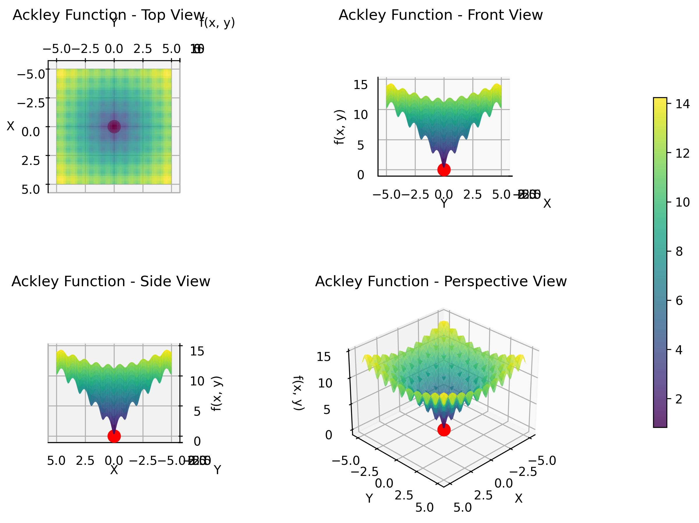
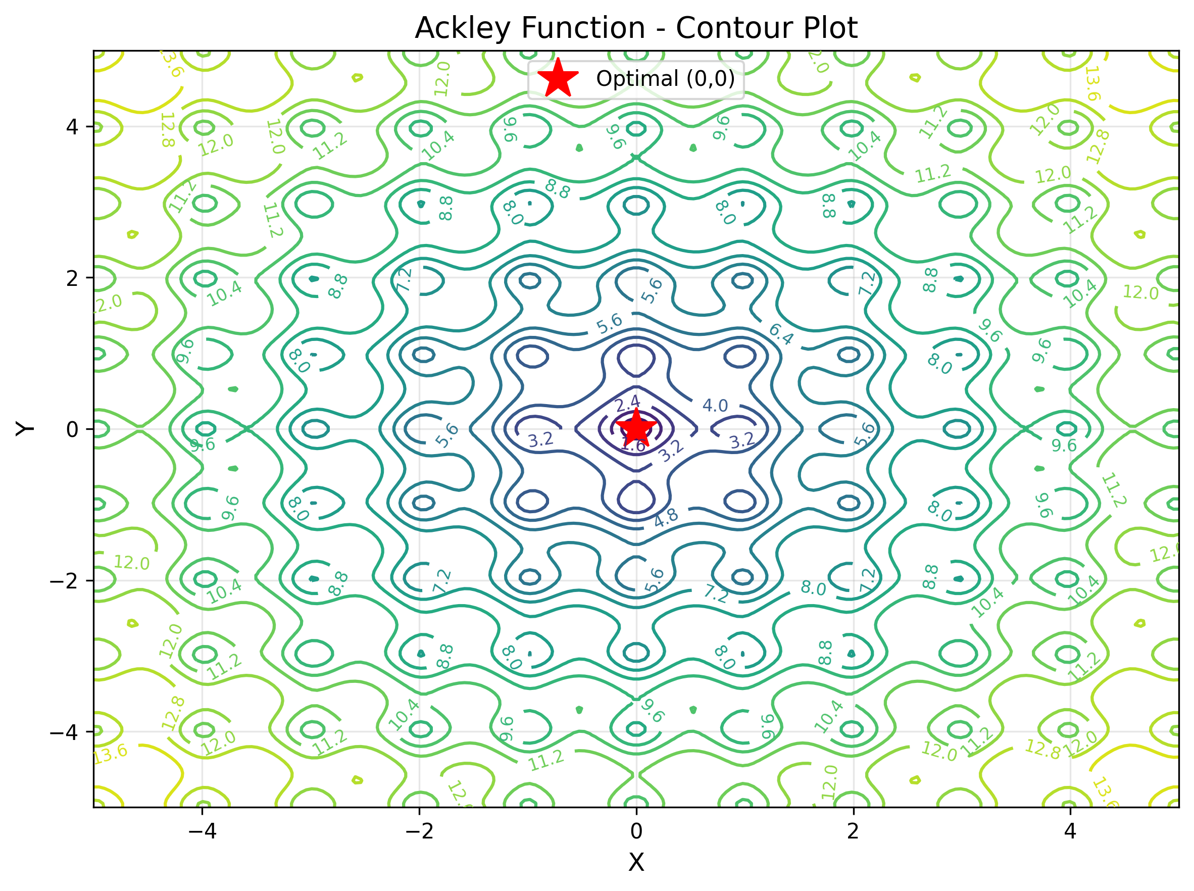
Ackley Function

The Ackley function is a widely used benchmark for testing global optimization algorithms. It features a complex multimodal landscape with many local minima surrounding a single global minimum at the origin. The function combines exponential and cosine components to create a nearly flat outer region with a sharp central peak, making it challenging for algorithms to locate the global optimum. This function simulates optimization problems in signal processing, neural network training, and parameter tuning where numerous local optima can trap search algorithms.

Key characteristics:

• Multimodal with many local minima
• Nearly flat outer region with exponential decay
• Sharp central peak around the global optimum
• Tests exploration vs exploitation balance

This objective function is expressed by the following formula.

$f(x) = -20 \exp\left(-0.2\sqrt{\frac{1}{n}\sum_{i=1}^{n}x_i^2}\right) - \exp\left(\frac{1}{n}\sum_{i=1}^{n}\cos(2\pi x_i)\right) + 20 + e$

The objective function is displayed in 3D as follows.

The contour display makes it easy to understand the value of the objective function. The star position indicates the optimal value.

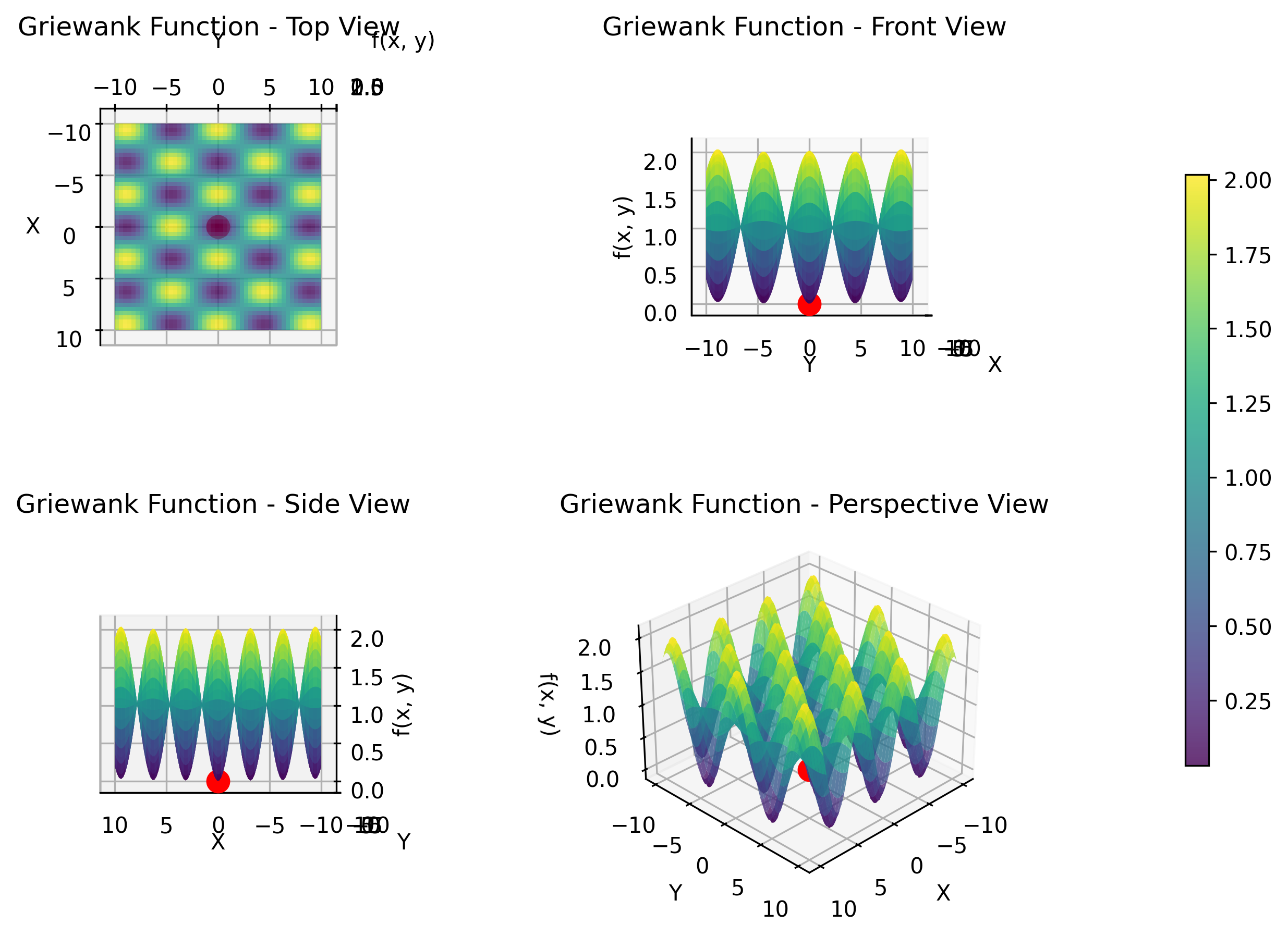
Griewank Function

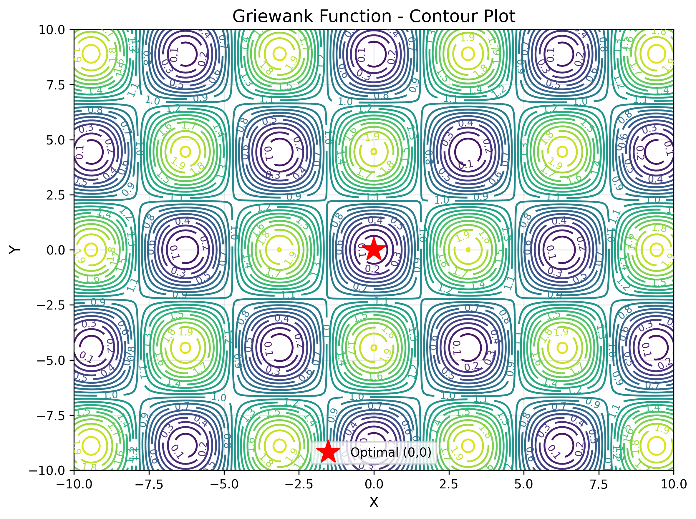
The Griewank function is a multimodal test function that becomes increasingly difficult as the number of dimensions increases. It features one global minimum at the origin and many local minima created by the interaction between quadratic and cosine components. The cosine term creates periodic structures that become more complex in higher dimensions. This function represents optimization challenges in engineering design, where multiple design variables interact to create complex landscapes with many feasible but suboptimal solutions.

Key characteristics:

• Difficulty increases with dimensionality
• Interaction between quadratic and periodic components
• Many local minima with single global optimum
• Tests algorithm scalability with problem size

This objective function is expressed by the following formula.

$f(x) = \frac{1}{4000}\sum_{i=1}^{n}x_i^2 - \prod_{i=1}^{n}\cos\left(\frac{x_i}{\sqrt{i}}\right) + 1$

The objective function is displayed in 3D as follows.

The contour display makes it easy to understand the value of the objective function. The star position indicates the optimal value.

Rastrigin Function

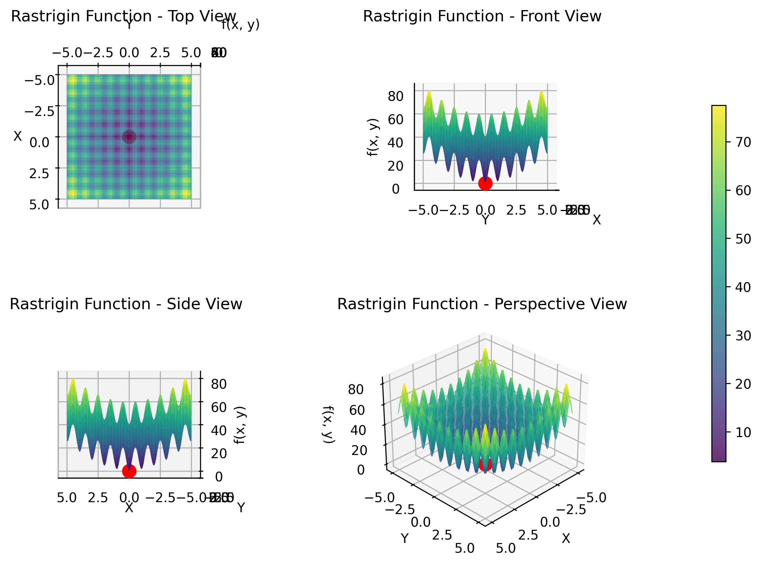
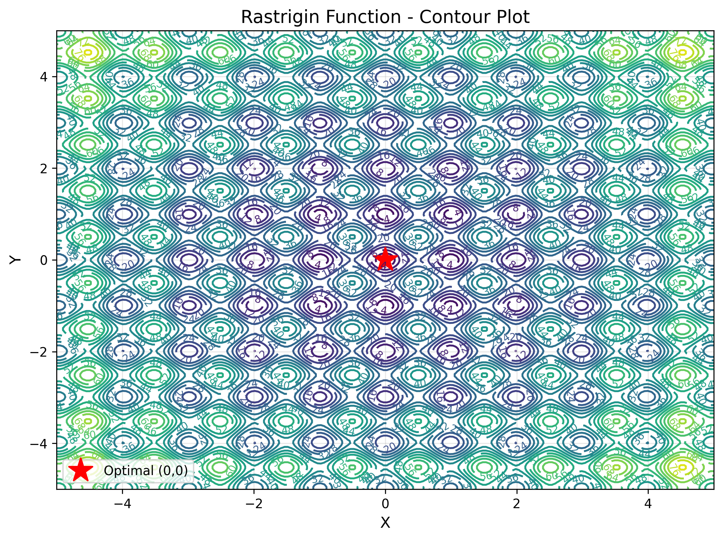
The Rastrigin function is a highly multimodal function characterized by many local minima arranged in a regular pattern. It is based on the sphere function with added cosine modulation that creates multiple peaks and valleys throughout the search space. This function is particularly challenging because it has a large number of local minima, making it difficult for algorithms to escape local optima and find the global minimum. It represents optimization problems in machine learning hyperparameter tuning, where many parameter combinations yield locally optimal but globally suboptimal results.

Key characteristics:

• Highly multimodal with regular pattern of local minima
• Based on sphere function with cosine modulation
• Large number of evenly distributed local optima
• Tests algorithm's ability to escape local minima

This objective function is expressed by the following formula.

$f(x) = 10n + \sum_{i=1}^{n}[x_i^2 - 10\cos(2\pi x_i)]$

The objective function is displayed in 3D as follows.

The contour display makes it easy to understand the value of the objective function. The star position indicates the optimal value.

Rosenbrock Function

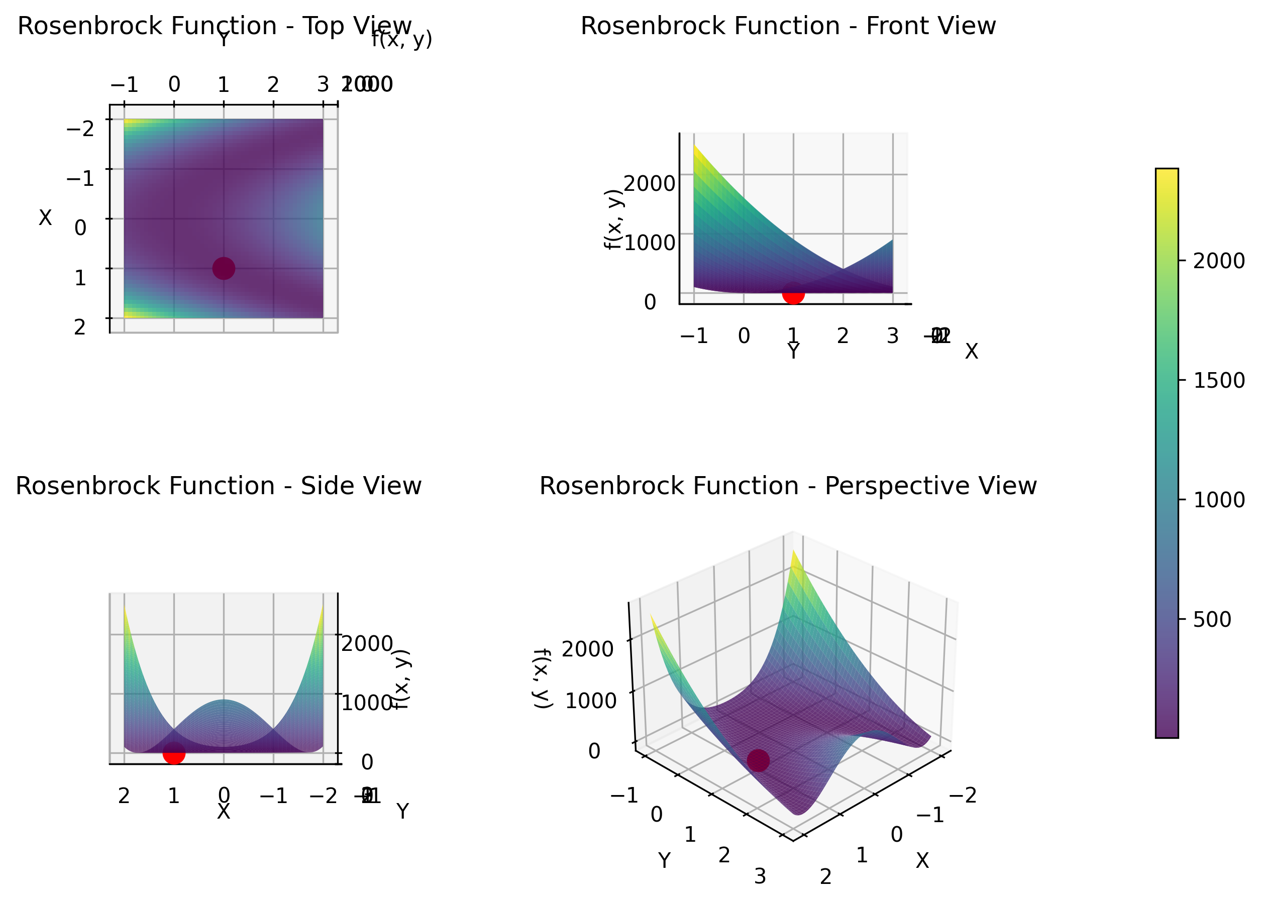
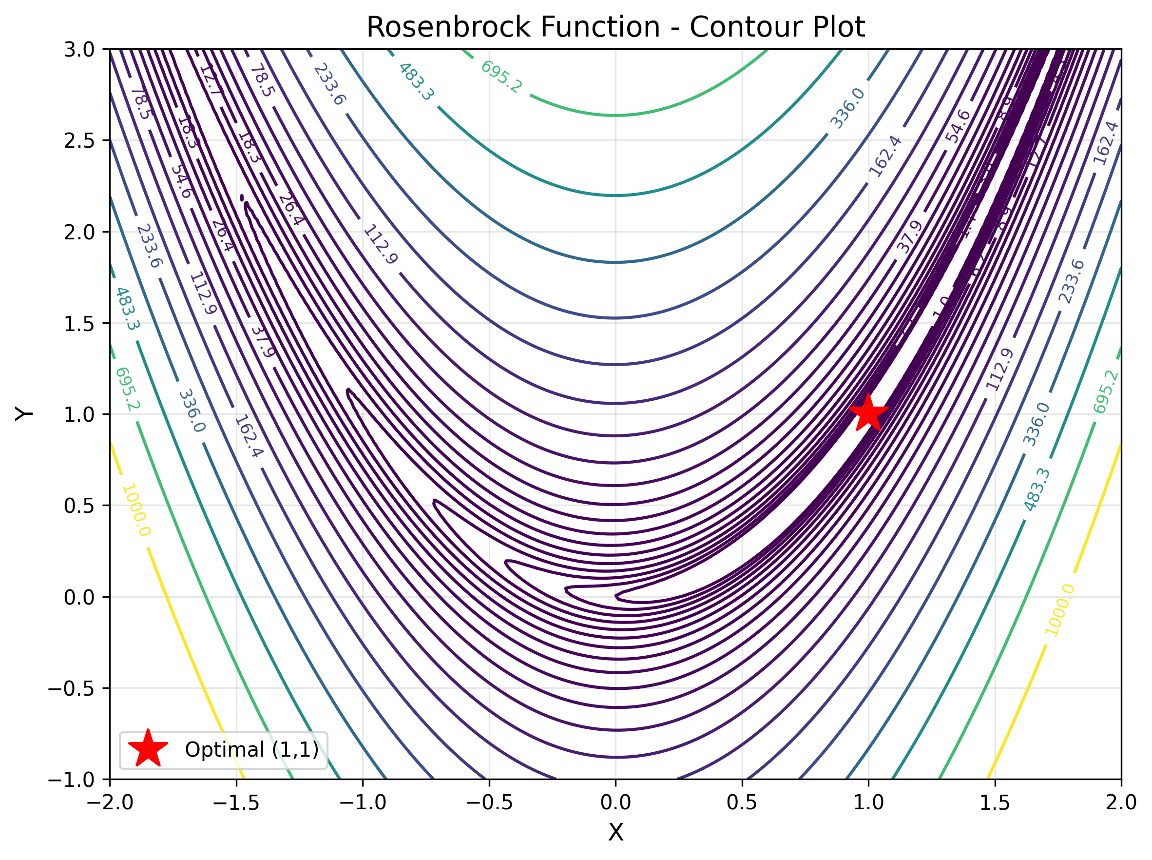
The Rosenbrock function, also known as the "banana function," is a classic optimization benchmark featuring a curved valley shape. While it has only one global minimum, the function is non-convex with a narrow, curved valley that is difficult for algorithms to navigate efficiently. The optimum lies in a long, narrow valley where one coordinate must be the square of the other. This function simulates optimization challenges in structural engineering and economics, where optimal solutions lie along constrained paths or relationships between variables.

Key characteristics:

• Non-convex with narrow, curved valley shape
• Single global minimum but difficult to locate
• Variables have quadratic relationship at optimum
• Tests algorithm's ability to follow curved paths

This objective function is expressed by the following formula.

$f(x) = \sum_{i=1}^{n-1}[100(x_{i+1} - x_i^2)^2 + (1 - x_i)^2]$

The objective function is displayed in 3D as follows.

The contour display makes it easy to understand the value of the objective function. The star position indicates the optimal value.

Schwefel Function

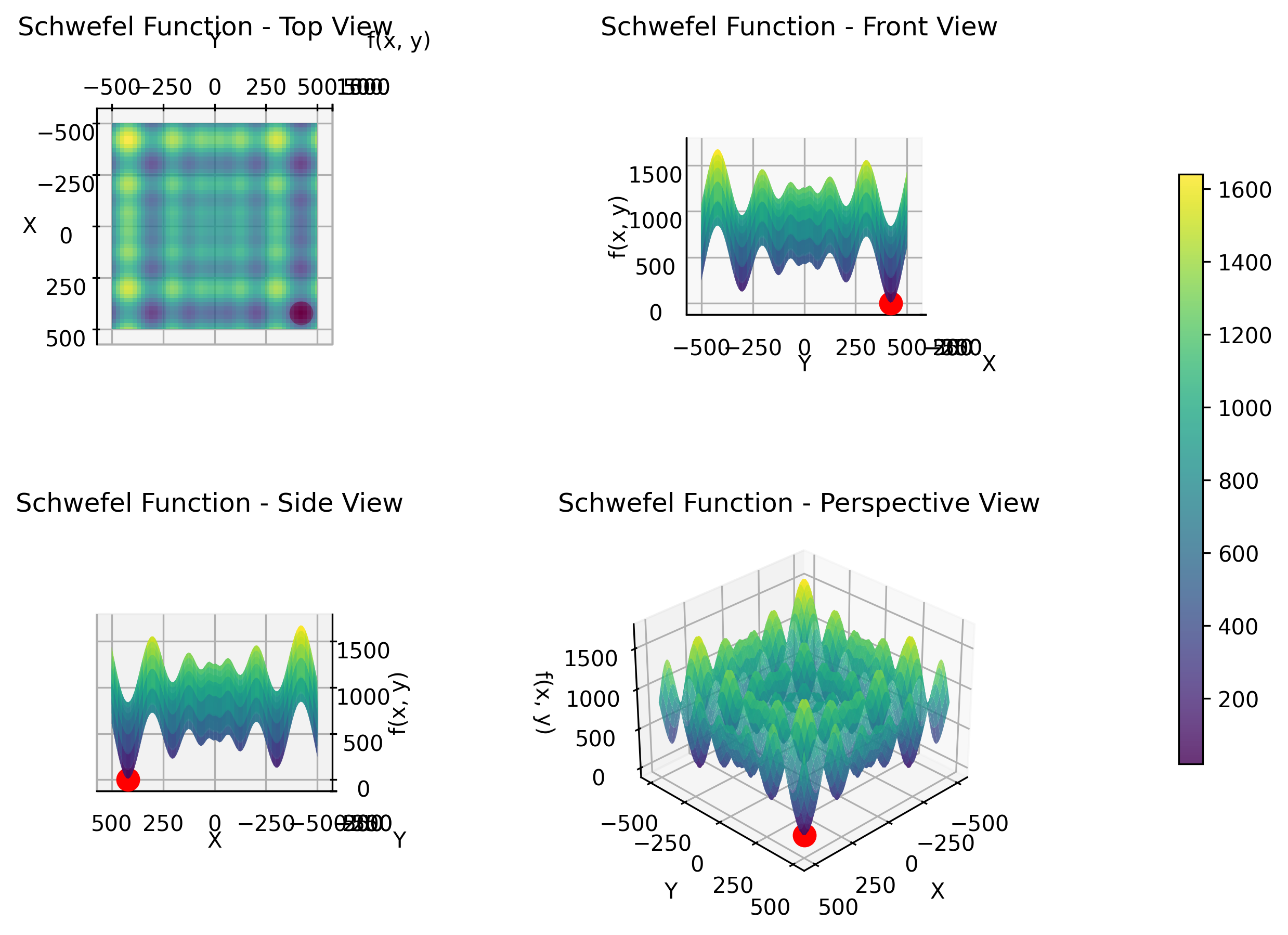
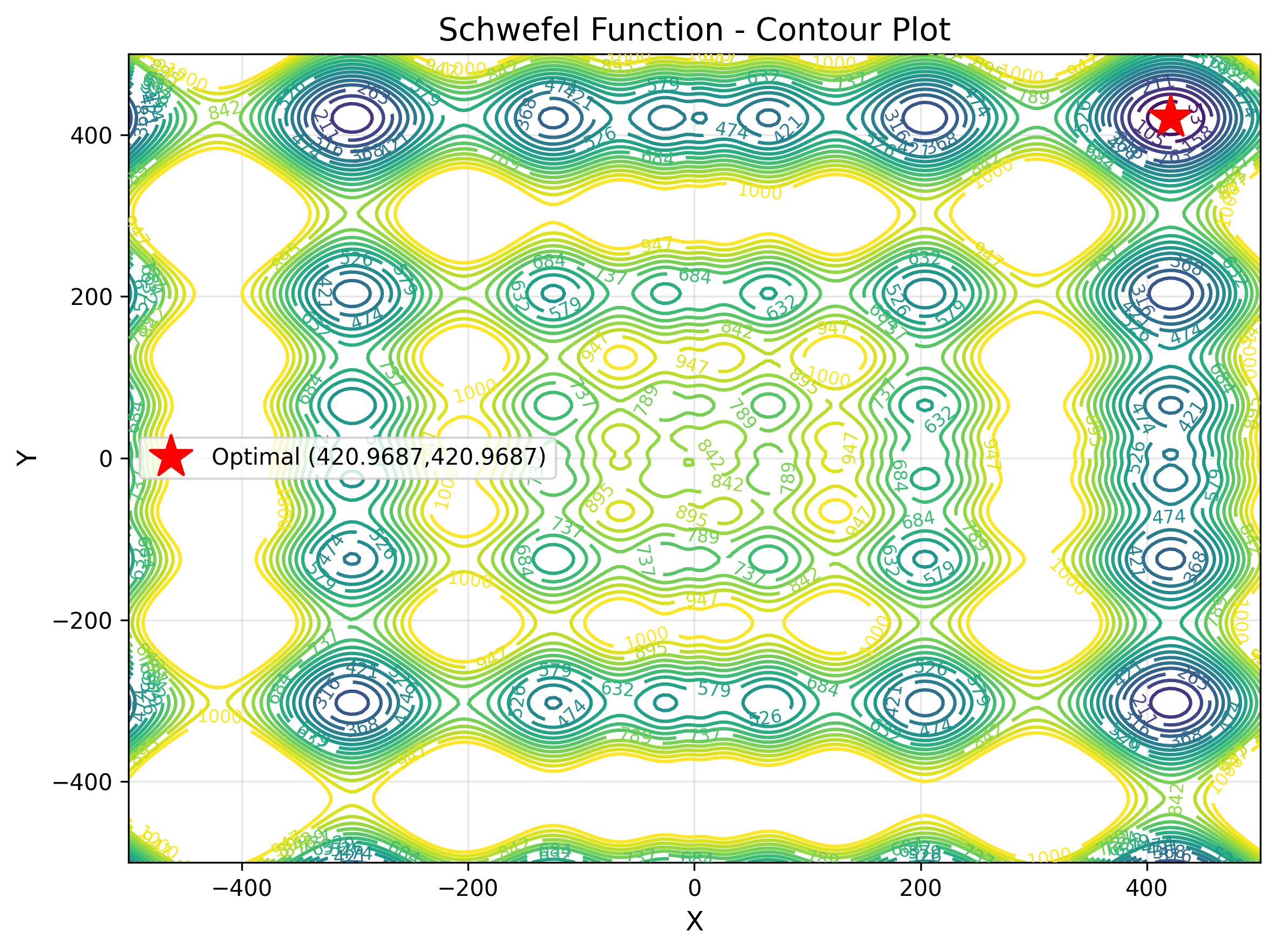
The Schwefel function is a deceptive multimodal function where the global minimum is far from the local minima, creating a challenging optimization landscape. The function features a complex structure with the global optimum located near the boundary of the search space, while many local minima are distributed throughout the interior. This deceptive nature makes it particularly difficult for algorithms that rely on gradient information or local search. It represents real-world problems in logistics and supply chain optimization, where the best solutions may be counterintuitive or located in unexpected regions of the solution space.

Key characteristics:

• Deceptive with global minimum far from local minima
• Global optimum near search space boundary
• Complex multimodal structure
• Tests algorithm's global exploration capability

This objective function is expressed by the following formula.

$f(x) = 418.9829n - \sum_{i=1}^{n}x_i\sin(\sqrt{|x_i|})$

The objective function is displayed in 3D as follows.

The contour display makes it easy to understand the value of the objective function. The star position indicates the optimal value.

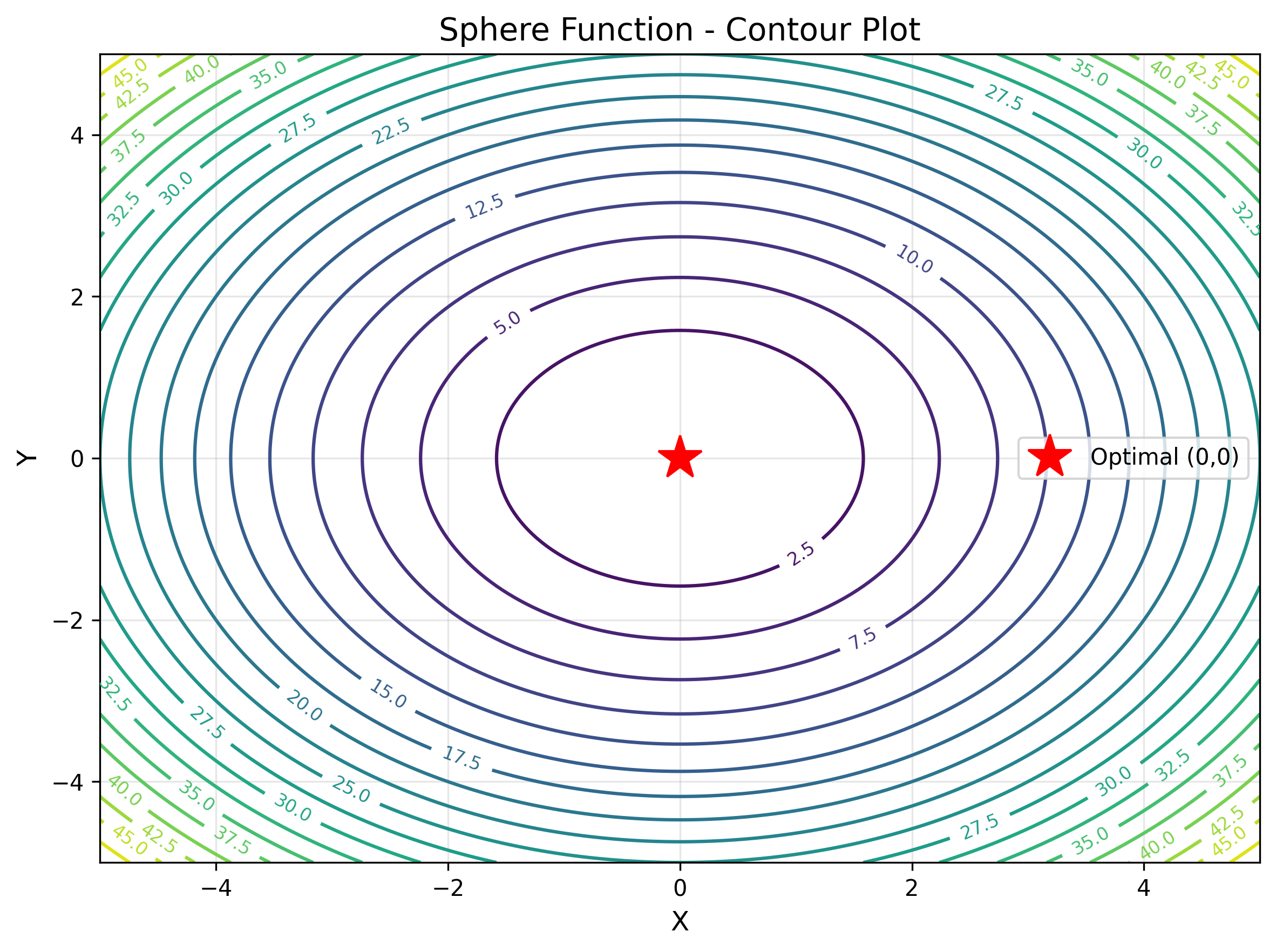
Sphere Function

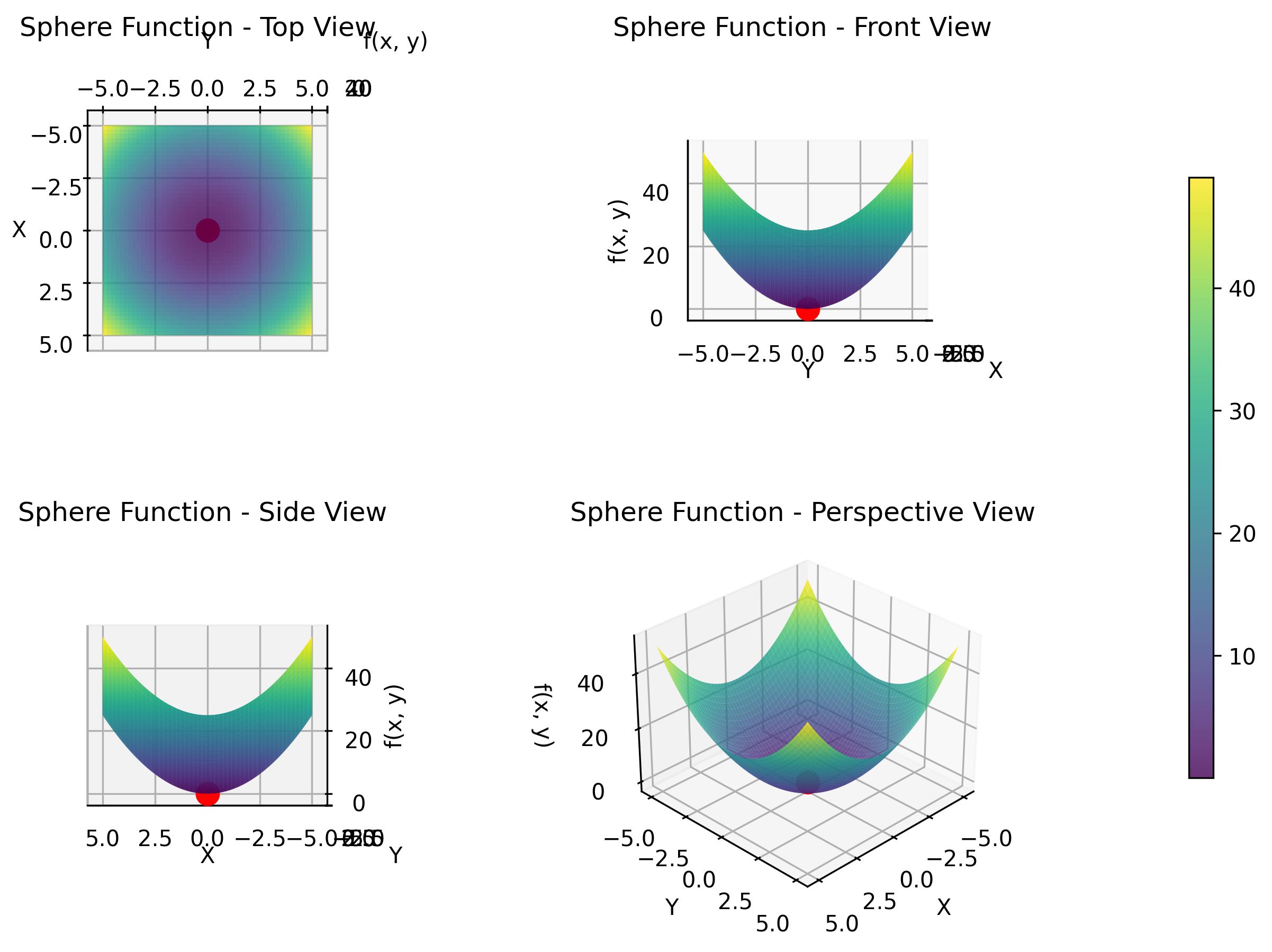
The Sphere function is the simplest and most fundamental benchmark function in optimization, featuring a single global minimum at the origin. It is unimodal and convex, making it relatively easy to optimize and ideal for testing basic algorithm performance and convergence speed. The function represents the sum of squares of all variables, creating a perfectly spherical contour in the solution space. This function simulates optimization problems in least squares fitting, calibration tasks, and any scenario where minimizing overall deviation or error is the primary objective.

Key characteristics:

• Unimodal and convex with single global minimum
• Perfectly spherical contours in solution space
• Simplest benchmark for algorithm testing
• Tests basic convergence speed and accuracy

This objective function is expressed by the following formula.

$f(x) = \sum_{i=1}^{n}x_i^2$

The objective function is displayed in 3D as follows.

The contour display makes it easy to understand the value of the objective function. The star position indicates the optimal value.