Random & Quasi-Monte Carlo

Tunny provides not only optimization algorithms such as Bayesian optimization and genetic algorithms, but also the Random Sampler and the QMC Sampler, which simply sample using random.
In this section, why they are in Tunny and when they are needed will be explained, including the technical details.

Difference between the two

Before reading the detailed explanation, it is best to first look at the results of sampling with each sampler for the best understanding.

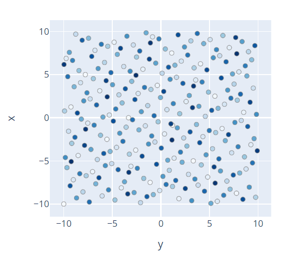
Since Tunny's Quasi-MonteCarlo sampler can use two algorithms, Halton and Sobol, these are the results of what values were sampled when x and y were sampled in the range of -10 to 10 using those two and a random sampler. In the following, 256 individuals were sampled, and the darker the color, the later they were sampled.

QMC(Halton)

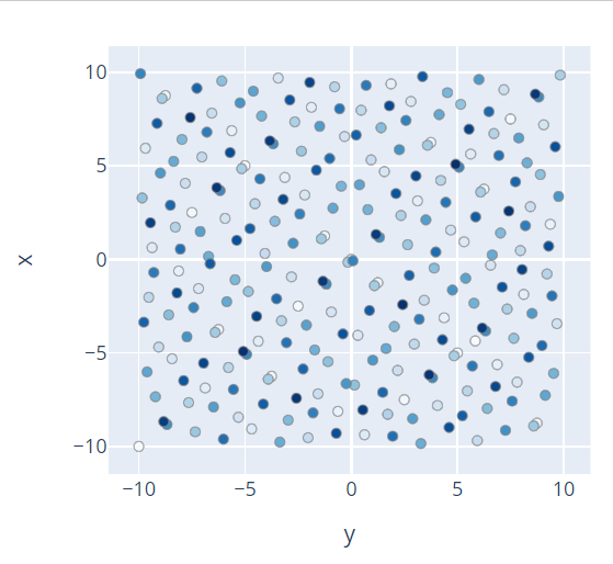
QMC(Sobol')

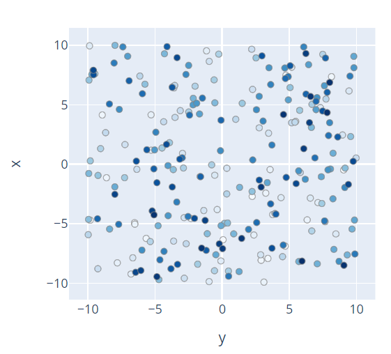
Random

I hope everyone who has seen these figures already understands the difference between Random and QMC.

Sampling with QMC is random, but the points are not crowded together in one place, and are sampled at moderate intervals. A number sequence with this characteristic is called a low-discrepancy sequence.

On the other hand, the Random Sampler is required to be as "random" as possible, as the word implies, so it may sample a point very close to a point that has already been observed.

Which to use?

If you want to know the entire solution space cleanly, I recommend using QMC.
The distinction between the use of Halton and Sobol' is that sobol has the feature of being able to sample with more variables, while still keeping a constant interval. However, Sobol' is an algorithm that results in a low-discrepancy sequence when sampling to powers of two, so Halton may be used if sampling to powers of two is not possible.

Next, let's look at when to use Random. Random is useful, for example, when the objective function may zigzag within a short range.
As explained above, QMC has low discrepancy, so there is always a fixed interval between the observation points. Therefore, zigzagging in a short range may not be observable.

Tunny allows you to change the range of variables within the same study. Thus, for example, you can start with QMC to check the entire study, and then change the range of the Number slider to sample only the areas you want to look at in more detail with Random. Using this functionality, it is possible to not only perform simple optimization, but also to gain a more detailed understanding of the solution space.

When to use it

As noted in the TPE and GP sections, these SMBOs (Sequential Model-Based Global Optimization) use Random in advance because the shape of the object to be optimized must generally be known prior to optimization.
SMBO is not the only one who should know this. When performing optimization, you yourself should know in advance whether the solution you seek is likely to exist within the range of the number slider you have set.
Random and QMC are used to achieve this.

As an example of how the solution space can be determined by the method, the results of 512 samplings for Random, QMC, and TPE, are shown below.

Random

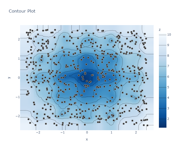
QMC(Sobol')

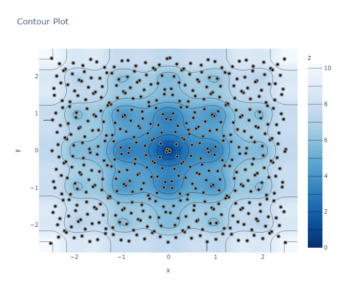
TPE

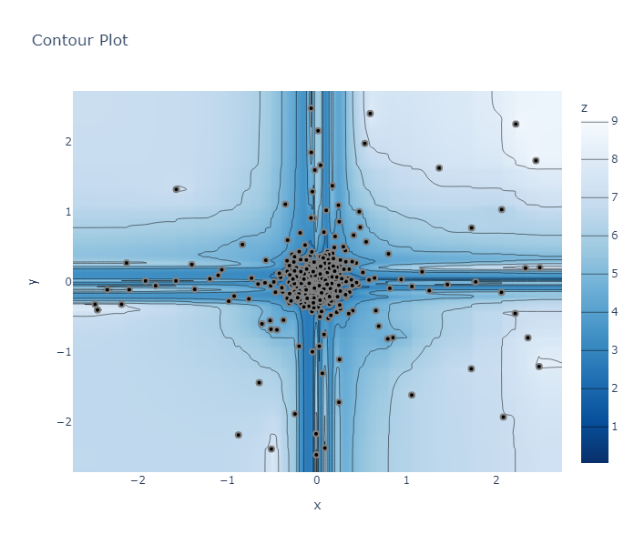
Did you find out what shape the objective function is?
This function is called the Ackley function and is expressed by the following equation.

# Ackley function
Z = -20*exp(-0.2*sqrt(0.5*(X^2 + Y^2))) - exp(0.5*(cos(2*pi*X) + cos(2*pi*Y))) + exp(1) + 20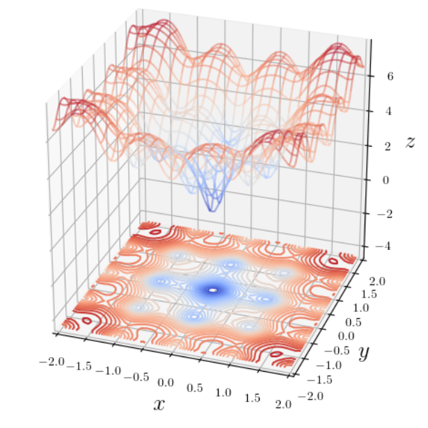

It is true that TPE solves this problem properly by taking a value close to 0, the global optimal solution, at (0,0), but the shape of the objective function is not as clear as with other methods.
It can be seen that the results with QMC are very close to the actual shapes.

As the above example shows, optimization only knows the best solution.
Random and QMC may not know the true optimal solution. However, by carefully analyzing the results, there is a possibility to obtain more information than the optimization.

For example, let's use the above example. Suppose you need a range of z-values less than or equal to 2. The optimization only shows that it will be approximately 0 near (0, 0). However, by using Random and QMC, you know that the range of -0.5 to 0.5 is below 2. In other words, you can know that the range of -0.5 to 0.5 is usable for this design, and you don't have to search the range around (0,0) again by yourself.

Reference

• scipy.stats.qmc
  • Tunny uses Scipy, a Python library, to calculate QMC.
• Low-discrepancy sequence
• Bergstra, James, and Yoshua Bengio. Random search for hyper-parameter optimization. Journal of machine learning research 13.2, 2012.